
外观
机器学习基础
Numpy
Numpy (Numerical Python) 是一个开源的 Python 科学计算库,用于快速处理任意维度的数组。
Numpy 支持常见的数组和矩阵操作。 对于同样的数值计算任务,使用 Numpy 比直接使用 Python 要简洁的多。
Numpy 使用 ndarray 对象来处理多维数组,该对象是一个快速而灵活的大数据容器。
Numpy 如何存储数据
Numpy 使用 ndarray 存储数据,类似 Python 原生的集合。
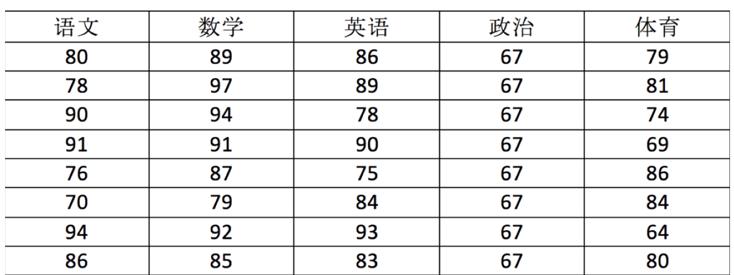
用 ndarray 进行存储:
import numpy as np

score = np.array(
[[80, 89, 86, 67, 79],
[78, 97, 89, 67, 81],
[90, 94, 78, 67, 74],
[91, 91, 90, 67, 69],
[76, 87, 75, 67, 86],
[70, 79, 84, 67, 84],
[94, 92, 93, 67, 64],
[86, 85, 83, 67, 80]])

print(score)
[[80 89 86 67 79]
[78 97 89 67 81]
[90 94 78 67 74]
[91 91 90 67 69]
[76 87 75 67 86]
[70 79 84 67 84]
[94 92 93 67 64]
[86 85 83 67 80]]ndarray 的属性
| 属性名字 | 属性解释 |
|---|---|
| ndarray.shape | 数组维度的元组 |
| ndarray.ndim | 数组维数 |
| ndarray.size | 数组中的元素数量 |
| ndarray.itemsize | 一个数组元素的长度 (字节) |
| ndarray.dtype | 数组元素的类型 |
| ndarray.nbytes | 数组总共的内存大小 |
# 接着前面的代码运行
print(f"score的形状为{score.shape}")
print(f"score的维度为{score.ndim}")
print(f"score的元素个数为{score.size}")
print(f"score的元素大小为{score.itemsize}")
print(f"score的内存大小为{score.nbytes}")
print(f"score的元素类型为{score.dtype}")
ndarray 的元素类型
新版 Numpy
| 名称 | 描述 | 简写/类型字符 |
|---|---|---|
| 布尔类型 | 逻辑真/假 (True/False) | bool_/? |
| 有符号整数 | 整数,按位宽区分 | int8 (i1),int16 (i2),int32 (i4),int64 (i8) |
| 默认整数 | 平台默认大小整数 (类似 C 的 long) | int_ (l) |
| 整数 (C) | C 标准类型对应的整数 | intc |
| 索引整数 | 用于数组索引的整数 | intp |
| 无符号整数 | 非负整数,对应位宽 | uint8 (u1),uint16 (u2),uint32 (u4),uint64 (u8) |
| 默认无符号整数 | 平台无符号整数 | uint |
| 无符号整数 (C) | C 标准类型对应的无符号整数 | uintc |
| 无符号索引整数 | 用于索引的无符号整数 | uintp |
| 浮点数 | 实数,精度按位宽 | float16 (f2),float32 (f4),float64 (f8) |
| 长双精度浮点数 | 扩展精度 (平台相关) | longdouble |
| 复数数值 | 实部和虚部为浮点 | complex64 (c8),complex128 (c16) |
| 长复数 | 扩展精度复数 | clongdouble |
| 字符串类型 | 固定长度字节字符串 | bytes_ (S) |
| Unicode 字符串 | 固定长度 Unicode | str_ (U) |
| Python 对象 | 任意 Python 对象 | object_ (O) |
| 日期时间类型 | 带单位的日期时间 | datetime64 |
| 时间差类型 | 带单位的时间间隔 | timedelta64 |
| 原始/空类型 | 原始内存块/结构化用 | void (V) |
旧版 Numpy
| 名称 | 描述 | 简写 |
|---|---|---|
| np.bool | 用一个字节存储的布尔类型 (True或False) | 'b' |
| np.int8 | tinyint 一个字节大小,-128 至 127 | 'i' |
| np.int16 | smallint 整数,-32768 至 32767 | 'i2' |
| np.int32 | int 整数,-2^31 至 2^32 -1 | 'i4' |
| np.int64 | bigint 整数,-2^63 至 2^63 - 1 | 'i8' |
| np.uint8 | tinyint unsigned 无符号整数,0 至 255 | 'u' |
| np.uint16 | smallint unsigned 无符号整数,0 至 65535 | 'u2' |
| np.uint32 | 无符号整数,0 至 2^32 - 1 | 'u4' |
| np.uint64 | 无符号整数,0 至 2^64 - 1 | 'u8' |
| np.float16 | 半精度浮点数: 16 位,正负号 1 位,指数 5 位,精度 10 位 | 'f2' |
| np.float32 | float 单精度浮点数: 32 位,正负号 1 位,指数 8 位,精度 23 位 | 'f4' |
| np.float64 | double 双精度浮点数: 64 位,正负号 1 位,指数 11 位,精度 52 位 | 'f8' |
| np.complex64 | 复数,分别用两个 32 位浮点数表示实部和虚部 | 'c8' |
| np.complex128 | 复数,分别用两个 64 位浮点数表示实部和虚部 | 'c16' |
| np.object_ | python 对象 | 'O' |
| np.string_ | 字符串 | 'S' |
| np.unicode_ | unicode 类型 (字符串) | 'U' |
标粗的是常用类型。
np.string_只支持 ASCII 编码,不支持 Unicode,而np.unicode_支持 Unicode 字符。
np.string_更适合处理旧有的二进制数据,而np.unicode_更适合处理现代文本数据。
若不指定,整数默认 int64,小数默认 float64。
Numpy 模块生成数组
生成 0 和 1 的数组
np.ones(shape, dtype)、np.ones_like(a, dtype): 用于创建一个与数组 a 形状相同且所有元素都为 1 的数组的函数。np.zeros(shape, dtype)、np.zeros_like(a, dtype): 用于创建一个与数组 a 形状相同且所有元素都为 0 的数组的函数。
ones = np.ones([4,8])
ones
array([[1., 1., 1., 1., 1., 1., 1., 1.],
[1., 1., 1., 1., 1., 1., 1., 1.],
[1., 1., 1., 1., 1., 1., 1., 1.],
[1., 1., 1., 1., 1., 1., 1., 1.]])从现有数组生成
np.array(object, dtype): 从现有的数组当中创建np.asarray(a, dtype): 相当于索引的形式,数组还是同一个
import numpy as np

a = np.array([[1, 2, 3], [4, 5, 6]])
a1 = np.array(a)
a2 = np.asarray(a)

print(a1)
print(a2)

print("-" * 20)
a[0][0] = 0

print(a1)
print(a2)
[[1 2 3]
[4 5 6]]
[[1 2 3]
[4 5 6]]
--------------------
[[1 2 3]
[4 5 6]]
[[0 2 3]
[4 5 6]]生成固定范围的数组
np.linspace(start, stop, num, endpoint): 创建等差数列。np.arange(start,stop, step, dtype): 类似于内置range函数。np.logspace(start, stop, num): 创建等比数列。
import numpy as np

a1 = np.linspace(1, 10, 2)
print(a1)

a2 = np.logspace(1, 4, 4, base=2)
print(a2)

a3 = np.arange(1, 10, 2)
print(a3)
[ 1. 10.]
[ 2. 4. 8. 16.]
[1 3 5 7 9]生成随机数组
np.random.rand(d1, d2,..., dn): 生成一个形状为 (d1, d2,..., dn) 的数组,里面的数都是 0~1 之间的均匀分布随机数。np.random.randint(start, end, shape): 生成给定形状的数组,里面的数在 start, end 之间。np.random.randn(*shape): 生成符合标准正态分布的随机数。
import numpy as np

# 生成一个 [0.0, 1.0) 之间的均匀分布的随机浮点数
rand_num = np.random.rand()
print("均匀分布的随机浮点数:", rand_num)

# 生成一个形状为(3, 2)的均匀分布的随机浮点数组
rand_array = np.random.rand(3, 2)
print("均匀分布的随机数组:\n", rand_array)

# 生成一个 [0, 100) 之间的均匀分布的随机整数数组
rand_num = np.random.randint(0, 100, size=(3, 2))
print("均匀分布的随机整数数组:\n", rand_num)
均匀分布的随机浮点数: 0.9980889637278122
均匀分布的随机数组:
[[0.83539653 0.40084522]
[0.74816643 0.80070457]
[0.01276914 0.68486665]]
均匀分布的随机整数数组:
[[73 77]
[29 31]
[64 87]]索引和切片
ndarray 的索引和切片和 Python 原生的列表方式一样,也可以按行和列操作,语法是 [:, :],类似于 Python 原生列表的 [:][:]。
import numpy as np

# 创建一个 3x4 的数组
arr = np.array([[1, 2, 3, 4],
                [5, 6, 7, 8],
                [9, 10, 11, 12]])

# 提取第 1 行和第 2 行的所有列
sub_array = arr[0:2, :]
print("第1行和第2行的所有列:\n", sub_array)

# 提取第 2 列和第 3 列的所有行
sub_array = arr[:, 1:3]
print("第2列和第3列的所有行:\n", sub_array)

# 提取第 1 行第 2 列到第 3 列的元素
sub_array = arr[0, 1:3]
print("第1行第2列到第3列的元素:", sub_array)
第 1 行和第 2 行的所有列:
[[1 2 3 4]
[5 6 7 8]]
第 2 列和第 3 列的所有行:
[[ 2 3]
[ 6 7]
[10 11]]
第 1 行第 2 列到第 3 列的元素: [2 3]修改形状
ndarray.reshape(shape, order): 返回一个具有相同数据域,但 shape 不一样的视图. 行,列不进行互换。ndarray.resize(new_shape): 修改数组本身的形状 (需要保持元素个数前后相同),行,列不进行互换。ndarray.T: 转置。
它们一个是返回新数组,一个是在原数组的基本上更改。
import numpy as np

array = np.arange(10)
array = array.reshape(2, 5)
print(array)

array.resize(5, 2)
print(array)

print(array.T)
[[0 1 2 3 4]
[5 6 7 8 9]]
[[0 1]
[2 3]
[4 5]
[6 7]
[8 9]]
[[0 2 4 6 8]
[1 3 5 7 9]]类型修改
ndarray.astype(type): 返回修改了类型后的数组。type 可以传合法的字符串,如 'float32',也可以传 numpy 模块定义的类。ndarray.tobytes([order]): 构造包含数组中原始数据字节的 Python 字节。
为什么转二进制? 方便网络传输。
import numpy as np

array = np.arange(10)
print(f"修改前的dtype: {array.dtype}")

array = array.astype(np.float32)
print(f"修改后的dtype: {array.dtype}")

print("-" * 20)

arr = np.array([[[1, 2, 3], [4, 5, 6]], [[12, 3, 34], [5, 6, 7]]])
print(f"数组: {arr}, 形状: {arr.shape}, 类型: {arr.dtype}")
bytes = arr.tobytes()
print(f"转成字节后的大小: {len(bytes)}")

arr = np.frombuffer(bytes, dtype=np.int64).reshape(2, 2, 3)
print(f"从字节转成数组: {arr}")
修改前的 dtype: int64
修改后的 dtype: float32
--------------------
数组: [[[ 1 2 3]
[ 4 5 6]]
[[12 3 34]
[ 5 6 7]]], 形状: (2, 2, 3), 类型: int64
转成字节后的大小: 96
从字节转成数组: [[[ 1 2 3]
[ 4 5 6]]
[[12 3 34]
[ 5 6 7]]]转成字节前后,要保持数据类型和形状一致。
去重
np.unique(ndarray)
import numpy as np

array = np.array([[1, 1, 2, 3], [4, 5, 5, 6]])
array = np.unique(array)
print(f"去重后的数组: {array}")
去重后的数组: [1 2 3 4 5 6]运算
加减乘除
可直接使用 Python 内置的加减乘除,取余,乘方等运算符。
import numpy as np

array1 = np.array([1, 2, 3, 4, 5, 6])
array2 = np.array([2, 3, 4, 5, 6, 7])

print(f"array1 + array2 = {array1 + array2}")
print(f"array1 * array2 = {array1 * array2}")
print(f"array1 ** 2 = {array1 ** 2}")
print(f"array1和array2的矩阵相乘 = {array1 @ array2}")
array1 + array2 = [ 3 5 7 9 11 13]
array1 * array2 = [ 2 6 12 20 30 42]
array1 ** 2 = [ 1 4 9 16 25 36]
array1 和 array2 的矩阵相乘 = 112
array1 和 array2 的点积 = 112逻辑运算
可用比较运算符,如大于小于,直接比较一个数。可直接使用赋值运算符和方括号改变符合条件的值。
import numpy as np

score = np.random.randint(40, 100, (3, 5))
print(f"随机生成的成绩: {score}")

print(f"大于等于60的成绩: {score[score >= 60]}")
print(f"每个成绩和60比较: {score >= 60}")
score[score >= 60] = 1
print(f"将大于等于60的成绩替换为1: {score}")
随机生成的成绩: [[97 53 88 44 59]
[66 89 65 68 47]
[98 86 94 75 41]]
大于等于 60 的成绩: [97 88 66 89 65 68 98 86 94 75]
每个成绩和 60 比较: [[ True False True False False]
[ True True True True False]
[ True True True True False]]
将大于等于 60 的成绩替换为 1: [[ 1 53 1 44 59]
[ 1 1 1 1 47]
[ 1 1 1 1 41]]通用判断函数
np.all(): 如果所有元素都满足条件,返回 True,否则返回 False。np.any(): 当你需要检查数组中是否至少有一个元素满足条件时使用,如果有一个元素满足条件,返回 True,否则返回 False。
import numpy as np

array = np.array([1, 2, 3, 4, 5, 6])

print(f"所有元素都大于5: {np.all(array >= 5)}")
print(f"所有元素都小于6: {np.all(array <= 6)}")
print(f"至少有一个元素大于5: {np.any(array > 5)}")
所有元素都大于 5: False
所有元素都小于 6: True
至少有一个元素大于 5: True
数组的余弦值: [ 0.54030231 -0.41614684 -0.9899925 -0.65364362 0.28366219 0.96017029]三元运算符
np.where(expression, a, b): 类似 Python 中的 if...else 结构。
# 判断前四名学生, 前四门课程中, 成绩中大于 60 的置为 1, 否则为 0
temp = score[:4, :4]
np.where(temp > 60, 1, 0)
复合逻辑需要结合 np.logical_and 和 np.logical_or 使用。
# 判断前四名学生, 前四门课程中, 成绩中大于 60 且小于 90 的换为 1, 否则为 0
np.where(np.logical_and(temp > 60, temp < 90), 1, 0)
# 判断前四名学生, 前四门课程中, 成绩中大于 90 或小于 60 的换为 1, 否则为 0
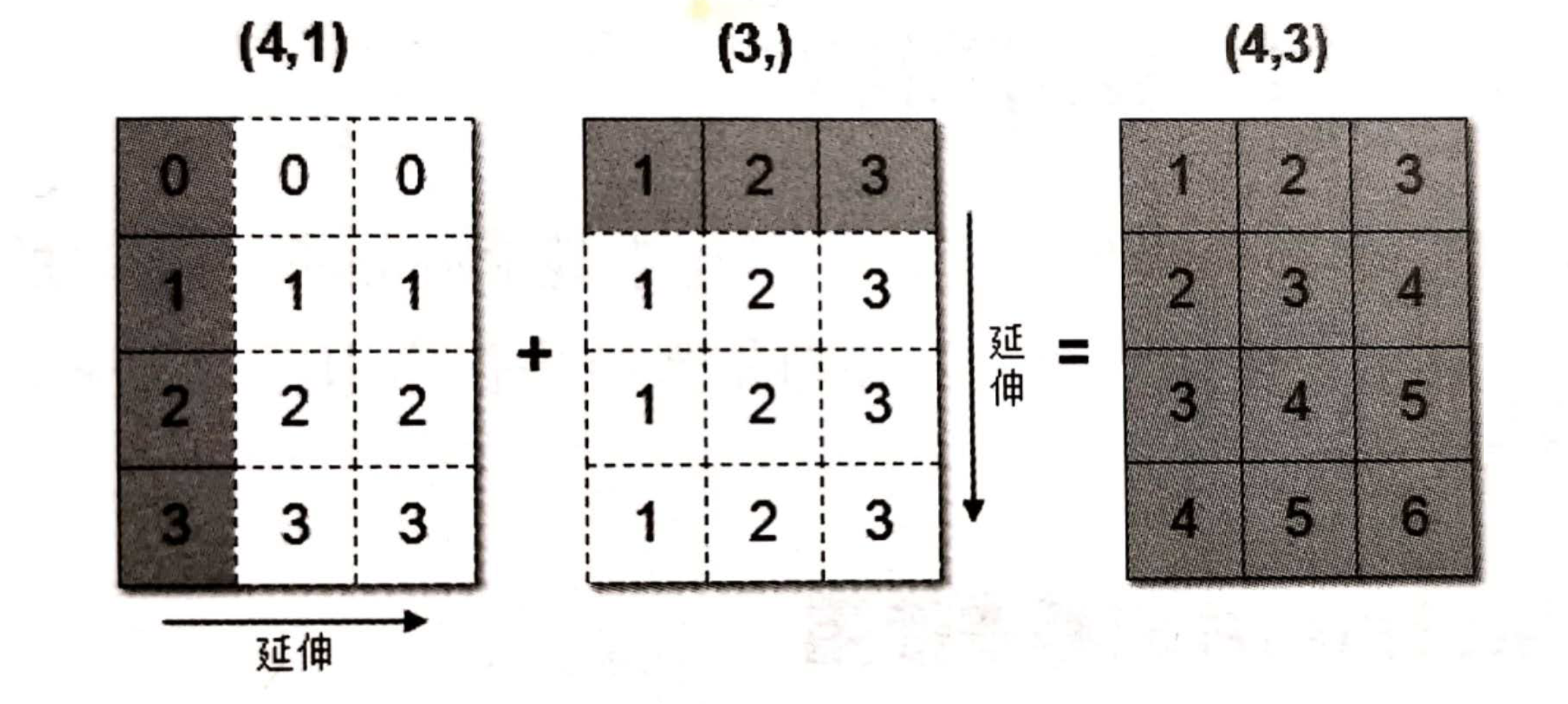
np.where(np.logical_or(temp > 90, temp < 60), 1, 0)数组的广播机制
数组在进行矢量化运算时,要求数组的形状是相等的. 当形状不相等的数组执行算术运算的时候,就会出现广播机制,该机制会对数组进行扩展,使数组的 shape 属性值一样,这样,就可以进行矢量化运算了。
arr1 = np.array([[0],[1],[2],[3]])  # 4 x 1
arr1.shape
# (4, 1)

arr2 = np.array([1,2,3])  # 1 x 3
arr2.shape
# (3,)

arr1+arr2
# 结果是:
array([[1, 2, 3],
       [2, 3, 4],
       [3, 4, 5],
       [4, 5, 6]])
上述代码中,数组 arr1 是 4 行 1 列,arr2 是 1 行 3 列。这两个数组要进行相加,按照广播机制会对数组 arr1 和 arr2 都进行扩展,使得数组 arr1 和 arr2 都变成 4 行 3 列。
统计运算
min(a, axis): 返回数组中的最小值。max(a, axis): 返回数组中的最大值。median(a, axis): 返回数组的中位数。mean(a, axis, dtype): 返回数组的平均数。std(a, axis, dtype): 返回数组的标准差。var(a, axis, dtype): 返回数组的方差。argmax(a, axis): 返回元素最大值的索引。argmin(a, axis): 返回元素最小值的索引。
import numpy as np

array = np.array([[1, 2, 3], [4, 5, 6]])
print(f"数组的最大值: {np.max(array)}")
print(f"数组的最小值: {np.min(array)}")
print(f"数组的中位数: {np.median(array)}")
print(f"数组的平均值: {np.mean(array)}")
print(f"数组的标准差: {np.std(array)}")
print(f"数组的方差: {np.var(array)}")
print(f"最小元素的下标: {np.argmin(array)}")
print(f"最大元素的下标: {np.argmax(array)}")
数组的最大值: 6
数组的最小值: 1
数组的中位数: 3.5
数组的平均值: 3.5
数组的标准差: 1.707825127659933
数组的方差: 2.9166666666666665
最小元素的下标: 0
最大元素的下标: 5以上方法,ndarray 对象也有,numpy 模块也会提供。如
numpy.min(array)相当于array.min()。
Pandas
Pandas 是 Python 的一个第三方包,也是商业和工程领域最流行的结构化数据工具集,用于数据清洗,处理以及分析。Pandas 底层是基于 Numpy 构建的,所以运行速度特别的快; 有专门的处理缺失数据的 API,具有强大而灵活的分组,聚合,转换功能。
基本使用
# 导入
import pandas as pd

# 从 CSV 文件读取数据集
df = pd.read_csv("data.csv")
print("查看数据集:", df, sep="\n", end="\n\n")
"""
      year   country           GDP
0     1960        美国  543300000000
1     1960        英国   73233967692
2     1960        法国   62225478000
3     1960        中国   59716467625
4     1960        日本   44307342950
...    ...       ...           ...
9925  2019  圣多美和普林西比     418637388
9926  2019        帕劳     268354919
9927  2019      基里巴斯     194647201
9928  2019        瑙鲁     118223430
9929  2019       图瓦卢      47271463

[9930 rows x 3 columns]
"""

# 查看前五行
print("查看前五行:", df.head(), sep="\n", end="\n\n")
"""
   year country           GDP
0  1960      美国  543300000000
1  1960      英国   73233967692
2  1960      法国   62225478000
3  1960      中国   59716467625
4  1960      日本   44307342950
"""

# 查询中国 GDP
print("查询中国GDP:", df[df["country"] == "中国"].head(10), sep="\n", end="\n\n")
"""
     year country          GDP
3    1960      中国  59716467625
107  1961      中国  50056868957
211  1962      中国  47209359005
316  1963      中国  50706799902
421  1964      中国  59708343488
525  1965      中国  70436266146
639  1966      中国  76720285969
755  1967      中国  72881631326
874  1968      中国  70846535055
993  1969      中国  79705906247
"""

# 将 year 设为索引
new_df = df.set_index("year")
print("将year设为索引:", new_df, sep="\n", end="\n\n")
"""
       country           GDP
year
1960        美国  543300000000
1960        英国   73233967692
1960        法国   62225478000
1960        中国   59716467625
1960        日本   44307342950
...        ...           ...
2019  圣多美和普林西比     418637388
2019        帕劳     268354919
2019      基里巴斯     194647201
2019        瑙鲁     118223430
2019       图瓦卢      47271463

[9930 rows x 2 columns]
"""

# 画出中国和日本的 GDP 折线图
jp_gdp = df[df.country=='日本'].set_index('year') # 按条件选取数据后, 重设索引
jp_gdp.GDP.plot()
china_gdp = df[df.country=='中国'].set_index('year') # 按条件选取数据后, 重设索引
china_gdp.GDP.plot()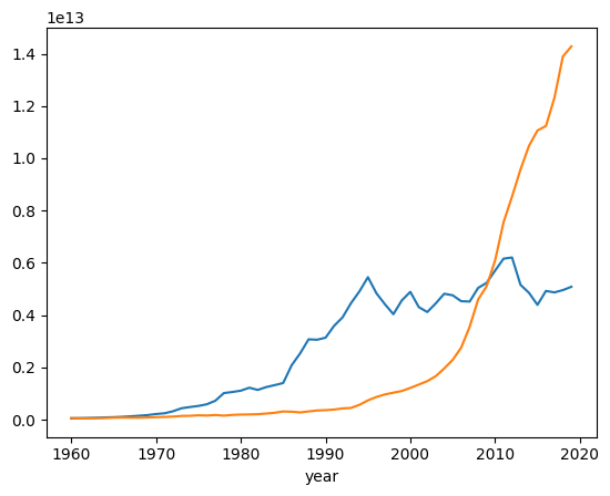
Pandas 数据结构与数据类型
Pandas 最核心的两个数据结构: DataFrame 和 Series。DataFrame 是表对象,Series 是列对象。
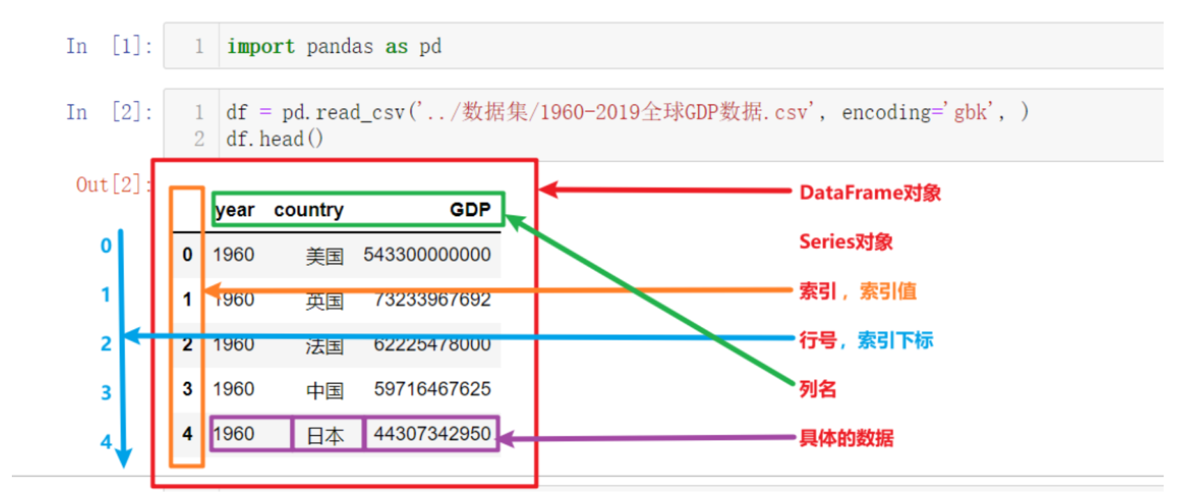
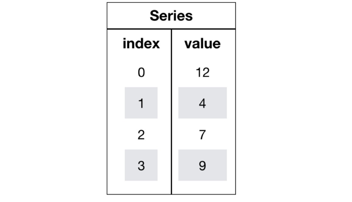
Series 对象
Series = index + values + dtype + name。DataFrame 的一列,本质上就是一个 Series。
创建 Series
通过 Python 原生列表创建,可使用自增索引或使用自定义索引。
import pandas as pd

# 使用默认自增索引
series1 = pd.Series([1, 2, 3, 4, 5])
print(series1)

# 自定义索引
series2 = pd.Series([1, 2, 3, 4, 5], index=['a', 'b', 'c', 'd', 'e'])
print(series2)
0 1
1 2
2 3
3 4
4 5
dtype: int64
a 1
b 2
c 3
d 4
e 5
dtype: int64使用字典或元组创建。
import pandas as pd

# 使用元组创建
series1 = pd.Series((1, 2, 3, 4, 5))
print(series1)

# 使用字典创建
series2 = pd.Series({
    'a': 1,
    'b': 2,
    'c': 3,
    'd': 4,
    'e': 5
})
print(series2)
0 1
1 2
2 3
3 4
4 5
dtype: int64
a 1
b 2
c 3
d 4
e 5
dtype: int64使用 numpy 创建。
import pandas as pd
import numpy as np

ndarray = np.array([1, 2, 3])
print(ndarray)
print(type(ndarray))

series = pd.Series(ndarray)
print(series)
print(type(series))
[1 2 3]
<class 'numpy.ndarray'>
0 1
1 2
2 3
dtype: int64
<class 'pandas.Series'>Series 常用属性
| 属性 | 说明 |
|---|---|
| index | 索引对象 |
| values | 底层数据 (ndarray) |
| dtypes | 数据类型 |
| shape | 形状 (由于是一维, 通常显示为(n,) ) |
| size | 元素个数 |
| ndim | 维度数 (永远是1) |
| name | Series 名称 |
| axes | 轴信息, 等价于 [index] |
| nbytes | 数据占用字节数 |
| flags | 内部标志信息 |
import pandas as pd
import numpy as np

ndarray = np.array([1, 2, 3, 4])
series = pd.Series(ndarray)

print(f"索引: {series.index}")
print(f"元素: {series.values}")
print(f"数据类型: {series.dtypes}")
print(f"形状: {series.shape}")
print(f"元素数量: {series.size}")
print(f"维度: {series.ndim}")
print(f"名称: {series.name}")
print(f"轴信息: {series.axes}")
print(f"数据占用字节数: {series.nbytes}")
print(f"内部标志: {series.flags}")
索引: RangeIndex(start=0, stop=4, step=1)
元素: [1 2 3 4]
数据类型: int64
形状: (4,)
元素数量: 4
维度: 1
名称: None
轴信息: [RangeIndex(start=0, stop=4, step=1)]
数据占用字节数: 32
内部标志: <Flags(allows_duplicate_labels=True)>Series 可以通过索引返回数据。
import pandas as pd
import numpy as np

ndarray = np.array(["Apple", "Banana", "Cherry", "Date"])
series = pd.Series(ndarray, index=["a", "b", "c", "d"])

print(series.a) # Apple
print(series["b"]) # Banana
DataFrame 对象
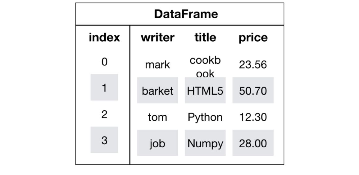
DataFrame 是一个类似于二维数组或表格 (如 Excel) 的对象,既有行索引,又有列索引。
- 行索引,表明不同行,横向索引,叫 index,0 轴,axis = 0
- 列索引,表名不同列,纵向索引,叫 columns,1 轴,axis = 1
创建 DataFrame
使用 pandas.read_csv() 函数。
import pandas as pd

df = pd.read_csv("data.csv")
print(df)
print(type(df))
year country GDP
0 1960 美国 543300000000
1 1960 英国 73233967692
2 1960 法国 62225478000
3 1960 中国 59716467625
4 1960 日本 44307342950
... ... ... ...
9925 2019 圣多美和普林西比 418637388
9926 2019 帕劳 268354919
9927 2019 基里巴斯 194647201
9928 2019 瑙鲁 118223430
9929 2019 图瓦卢 47271463
[9930 rows x 3 columns]
<class 'pandas.DataFrame'>使用字典加列表的方式创建。
import pandas as pd

df1_data = {
    '日期': ['2021-08-21', '2021-08-22', '2021-08-23'],
    '温度': [25, 26, 50],
    '湿度': [81, 50, 56]
}
df1 = pd.DataFrame(data=df1_data)
print(df1)
日期 温度 湿度
0 2021-08-21 25 81
1 2021-08-22 26 50
2 2021-08-23 50 56使用列表创建。
import pandas as pd

df2_data = [
    ('2021-08-21', 25, 81),
    ('2021-08-22', 26, 50),
    ('2021-08-23', 27, 56)
]

df2 = pd.DataFrame(
    data=df2_data,
    columns=['日期', '温度', '湿度'],
    index = ['row_1','row_2','row_3'] # 手动指定索引
)
print(df2)
日期 温度 湿度
row_1 2021-08-21 25 81
row_2 2021-08-22 26 50
row_3 2021-08-23 27 56- 使用 numpy 创建,这里不再演示。
- 在创建时可指定行索引和列索引。行索引通过 index 参数传入,列索引通过 columns 参数传入。
import pandas as pd
import numpy as np

score = np.random.randint(40, 100, (3, 2))
score_df = pd.DataFrame(score, index=["Row1", "Row2", "Row3"], columns=["Column1", "Column2"])
print(score_df)
Column1 Column2
Row1 61 84
Row2 63 74
Row3 86 85DataFrame 常用属性和方法
| 属性和方法 | 说明 |
|---|---|
| shape | 返回行列数量,格式为 (行数,列数) |
| index | 返回行索引对象 |
| columns | 返回列名 |
| values | 获取值,是一个 numpy 数组 |
| T | 转置 |
| head(n=5) | 获取前 n 行数据 |
| tail(n=5) | 显示后 n 行数据 |
import pandas as pd
import numpy as np

score = np.random.randint(40, 100, (5, 3))
score_df = pd.DataFrame(score, index=["Row1", "Row2", "Row3", "Row4", "Row5"], columns=["Column1", "Column2", "Column3"])
print(f"行列数: {score_df.shape}")
print(f"行索引对象: {score_df.index}")
print(f"列索引对象: {score_df.columns}")
print(f"值: {score_df.values}")
print(f"转置: {score_df.T}")
print(f"前三行: {score_df.head(3)}")
print(f"后两行: {score_df.tail(2)}")
行列数: (5, 3)
行索引对象: Index(['Row1', 'Row2', 'Row3', 'Row4', 'Row5'], dtype='str')
列索引对象: Index(['Column1', 'Column2', 'Column3'], dtype='str')
值: [[73 80 87]
[91 59 79]
[42 80 85]
[91 41 68]
[42 69 69]]
转置: Row1 Row2 Row3 Row4 Row5
Column1 73 91 42 91 42
Column2 80 59 80 41 69
Column3 87 79 85 68 69
前三行: Column1 Column2 Column3
Row1 73 80 87
Row2 91 59 79
Row3 42 80 85
后两行: Column1 Column2 Column3
Row4 91 41 68
Row5 42 69 69Pandas 的数据类型
| Pandas Dtype | 说明 | 典型对应的 Python 类型/备注 |
|---|---|---|
| int64, Int64 | 整数类型 | Python int; 其中 Int64 是可空整数 (允许缺失值 pd.NA) |
| float64/float32/… | 浮点数 | Python float; 缺失值通常为 np.nan |
| bool/boolean | 布尔类型 | Python bool (True/False); boolean 是可空布尔类型, 允许 pd.NA |
| object | 通用 Python 对象 | 任意 Python 对象 (最常见是字符串 str) |
| string | Pandas 专用字符串类型 | Python str 或 pd.NA (比 object 更严格, 更优化) |
| datetime64[ns] | 不带时区的日期时间 | Python datetime.datetime/pd.Timestamp |
| datetime64[ns, tz] | 带时区的日期时间 | Python datetime.datetime (带 tzinfo)/pd.Timestamp |
| timedelta64[ns] | 时间差 | Python datetime.timedelta/pd.Timedelta |
| category | 分类类型 | Python 原生无特定类型, 但可映射为分类标签值 (节省内存) |
| 扩展类型 | 扩展 dtype (不是基本 NumPy dtype) | 说明/对应 Python 类型 |
|---|---|---|
| PeriodDtype | 周期数据 (如年份/月份/季度) | Python pandas.Period |
| IntervalDtype | 区间类型 (数值区间) | Python pandas.Interval |
| SparseDtype | 稀疏数据类型 (节省大量空值内存) | 对应稀疏数组 |
| ArrowDtype (如 string[pyarrow]) | 基于 Apache Arrow 的高效存储 | Python 标量或 pd.NA (实验性/高效内存格式) |
Pandas 基本操作
索引操作
可直接使用行列索引获取某一单元的值 (先列后行)。
import pandas as pd
import numpy as np

score = np.random.randint(40, 100, (5, 3))
score_df = pd.DataFrame(score, index=["Row1", "Row2", "Row3", "Row4", "Row5"], columns=["Column1", "Column2", "Column3"])
print(score_df["Column3"])
print(score_df["Column1"]["Row1"])

# 错误的操作: score_df["Row1"]["Column1"]
# 错误的操作: score_df[0][0]
Row1 99
Row2 95
Row3 57
Row4 90
Row5 98
Name: Column3, dtype: int32
49可以结合 loc 或者 iloc 使用索引,使用前者只能使用行列索引,且是先行后列,使用后者可以使用下标。
import pandas as pd
import numpy as np

score = np.random.randint(40, 100, (5, 3))
score_df = pd.DataFrame(score, index=["Row1", "Row2", "Row3", "Row4", "Row5"], columns=["Column1", "Column2", "Column3"])

print(score_df.loc["Row1"])
print(score_df.loc["Row1", "Column2"])
print(score_df.loc["Row1":"Row3", "Column2"])

print(score_df.iloc[0])
print(score_df.iloc[0, 1])
print(score_df.iloc[0:3, 1])
Column1 69
Column2 45
Column3 72
Name: Row1, dtype: int32
45
Row1 45
Row2 54
Row3 68
Name: Column2, dtype: int32
Column1 69
Column2 45
Column3 72
Name: Row1, dtype: int32
45
Row1 45
Row2 54
Row3 68
Name: Column2, dtype: int32通过一层索引名,可以修改一整列的值; 不可以通过两层索引,修改某个单元格的值。
import pandas as pd
import numpy as np

score = np.random.randint(40, 100, (5, 3))
score_df = pd.DataFrame(score, index=["Row1", "Row2", "Row3", "Row4", "Row5"], columns=["Column1", "Column2", "Column3"])

score_df["Column1"] = 1
print(score_df)

score_df["Column4"] = score_df["Column1"] + score_df["Column2"] + score_df["Column3"]
print(score_df)

# score_df["Column1", "Row1"] = -100  # 错误
# score_df["Column1"]["Row1"] = -100  # 错误
score_df.loc["Row1", "Column1"] = -100
print(score_df)
Column1 Column2 Column3
Row1 1 83 96
Row2 1 87 51
Row3 1 93 80
Row4 1 91 58
Row5 1 83 80
Column1 Column2 Column3 Column4
Row1 1 83 96 180
Row2 1 87 51 139
Row3 1 93 80 174
Row4 1 91 58 150
Row5 1 83 80 164
Column1 Column2 Column3 Column4
Row1 -100 83 96 180
Row2 1 87 51 139
Row3 1 93 80 174
Row4 1 91 58 150
Row5 1 83 80 164修改行索引对象和列索引对象,通过直接给 index 对象和 columns 对象赋值。
import pandas as pd
import numpy as np

score = np.random.randint(40, 100, (5, 3))
score_df = pd.DataFrame(score, index=["Row1", "Row2", "Row3", "Row4", "Row5"], columns=["Column1", "Column2", "Column3"])

print(score_df.index)
print(score_df.columns)

score_df.index = ["行1", "行2", "行3", "行4", "行5"]
score_df.columns = ["列A", "列B", "列C"]

print(score_df.index)
print(score_df.columns)
Index(['Row1', 'Row2', 'Row3', 'Row4', 'Row5'], dtype='str')
Index(['Column1', 'Column2', 'Column3'], dtype='str')
Index(['行1', '行2', '行3', '行4', '行5'], dtype='str')
Index(['列A', '列B', '列C'], dtype='str')可以通过 set_index 方法设置行索引。
import pandas as pd
import numpy as np

score = np.random.randint(40, 100, (5, 3))
score_df = pd.DataFrame(score, index=["Row1", "Row2", "Row3", "Row4", "Row5"], columns=["Column1", "Column2", "Column3"])

print(score_df)

score_df.set_index("Column1", inplace=True)

print(score_df)
Column1 Column2 Column3
Row1 93 77 79
Row2 95 98 78
Row3 76 69 51
Row4 75 63 83
Row5 95 88 54
Column2 Column3
Column1
93 77 79
95 98 78
76 69 51
75 63 83
95 88 54添加删除列
添加列,使用 df["new_col"] = ['value1',...] 的语法即可。
import pandas as pd

# 构造一个索引和数据都"故意打乱"的DataFrame
df = pd.DataFrame({
    "姓名": ["张三", "李四", "王五", "赵六"],
    "分数": [88, 92, 75, 92],
    "年龄": [20, 19, 21, 18]
}, index=[3, 1, 4, 2])

print("原始DataFrame: ")
print(df)

df['等级'] = [10, 9, 10, 9]
print("添加新列后的DataFrame: ")
print(df)
原始 DataFrame:
姓名 分数 年龄
3 张三 88 20
1 李四 92 19
4 王五 75 21
2 赵六 92 18
添加新列后的 DataFrame:
姓名 分数 年龄 等级
3 张三 88 20 10
1 李四 92 19 9
4 王五 75 21 10
2 赵六 92 18 9删除列,使用 drop 方法删除,可指定按行删除还是按列删除。如果按行删除,需指定 index 参数,如果是按列删除,需指定 columns 参数。
import pandas as pd

# 构造一个索引和数据都"故意打乱"的DataFrame
df = pd.DataFrame({
    "姓名": ["张三", "李四", "王五", "赵六"],
    "分数": [88, 92, 75, 92],
    "年龄": [20, 19, 21, 18]
}, index=[3, 1, 4, 2])

print("原始DataFrame: ")
print(df)

df['等级'] = [10, 9, 10, 9]
print("添加新列后的DataFrame: ")
print(df)

df.drop(columns=['等级'], inplace=True)
print("删除等级列后的DataFrame: ")
print(df)
原始 DataFrame:
姓名 分数 年龄
3 张三 88 20
1 李四 92 19
4 王五 75 21
2 赵六 92 18
添加新列后的 DataFrame:
姓名 分数 年龄 等级
3 张三 88 20 10
1 李四 92 19 9
4 王五 75 21 10
2 赵六 92 18 9
删除等级列后的 DataFrame:
姓名 分数 年龄
3 张三 88 20
1 李四 92 19
4 王五 75 21
2 赵六 92 18排序操作
df.sort_index(): 用索引排序。
import pandas as pd

data = {
    "姓名": ["张三", "李四", "王五"],
    "分数": [88, 92, 75]
}

df = pd.DataFrame(data, index=[3, 1, 2])

print("原始DataFrame: ")
print(df)

df_sorted = df.sort_index()

print("\n按索引排序后: ")
print(df_sorted)
原始 DataFrame:
姓名 分数
3 张三 88
1 李四 92
2 王五 75
按索引排序后:
姓名 分数
1 李四 92
2 王五 75
3 张三 88df.sort_index(by, axis=0, ascending=True, inplace=False): 通过 by 参数指定排序列,ascending 代表是否升序,如果是多列,就用列表指定每一列的顺序,inplace 代表是否替换源对象。
import pandas as pd

df = pd.DataFrame({
    "姓名": ["张三", "李四", "王五", "赵六"],
    "分数": [88, 92, 75, 92],
    "年龄": [20, 19, 21, 18]
}, index=[3, 1, 4, 2])

print("原始DataFrame: ")
print(df)

# ======================
# 按索引排序
# ======================
df_by_index = df.sort_index()

print("\n按索引排序 sort_index(): ")
print(df_by_index)

# ======================
# 按单列值排序
# ======================
df_by_score = df.sort_values(by="分数")

print("\n按分数排序 sort_values(by='分数'): ")
print(df_by_score)

# ======================
# 按多列值排序
# ======================
df_multi = df.sort_values(
    by=["分数", "年龄"],
    ascending=[False, True]
)

print("\n先按分数降序, 再按年龄升序: ")
print(df_multi)
原始 DataFrame:
姓名 分数 年龄
3 张三 88 20
1 李四 92 19
4 王五 75 21
2 赵六 92 18
按索引排序 sort_index():
姓名 分数 年龄
1 李四 92 19
2 赵六 92 18
3 张三 88 20
4 王五 75 21
按分数排序 sort_values(by='分数'):
姓名 分数 年龄
4 王五 75 21
3 张三 88 20
1 李四 92 19
2 赵六 92 18
先按分数降序,再按年龄升序:
姓名 分数 年龄
2 赵六 92 18
1 李四 92 19
3 张三 88 20
4 王五 75 21df.rank(axis=0, numeric_only=False, method='average', na_option='keep', ascending=True, pct=False): 用列值排序, 默认是升序。
axis: 默认是按行排序,如果是按列排序,则将 axis 设置为 1。numeric_only: 默认是 True,表示只对数字列排序,如果是 False,则对所有列排序。method: 默认是 average,表示平均值排序。'average': 平均值排序,相同值的排名取平均值。'min': 最小值排序,相同值的排名取最小值。'max': 最大值排序,相同值的排名取最大值。'dense': 排名一致,数值相同的评分一致。
na_option: 默认是 keep,表示保留缺失值。'keep': NaN 值保留原有位置。'top': NaN 值放在前面。'bottom': NaN 值放在后面。
ascending: 默认是 True,表示升序排序。pct: 默认是 False,表示不返回百分比排名。
获取 DataFrame 信息
describe()函数用于获取 DataFrame 每列的最小值,最大值,平均值,中位数,方差,标准差等信息。info()函数用于描述 DataFrame 的信息。
import pandas as pd

# 构造一个索引和数据都"故意打乱"的DataFrame
df = pd.DataFrame({
    "姓名": ["张三", "李四", "王五", "赵六"],
    "分数": [88, 92, 75, 92],
    "年龄": [20, 19, 21, 18]
}, index=[3, 1, 4, 2])

print(df.describe())
df.info()
分数 年龄
count 4.000000 4.000000
mean 86.750000 19.500000
std 8.057088 1.290994
min 75.000000 18.000000
25% 84.750000 18.750000
50% 90.000000 19.500000
75% 92.000000 20.250000
max 92.000000 21.000000
<class 'pandas.DataFrame'>
Index: 4 entries, 3 to 2
Data columns (total 3 columns):
# Column Non-Null Count Dtype
--- ------ -------------- -----
0 姓名 4 non-null str
1 分数 4 non-null int64
2 年龄 4 non-null int64
dtypes: int64(2), str(1)
memory usage: 128.0 bytesPandas 的运算
Pandas 的加减乘除
Pandas 可直接使用 Python 原生运算符计算,适用于 DataFrame 和 Series,也可使用 add,sub 等方法。
import pandas as pd

df1 = pd.DataFrame({
    "Col1": [1, 2, 3, 4, 5],
    "Col2": [6, 7, 8, 9, 10],
    "Col3": [11, 12, 13, 14, 15]
})
df2 = pd.DataFrame({
    "Col1": [16, 17, 18, 19, 20],
    "Col2": [21, 22, 23, 24, 25],
    "Col3": [26, 27, 28, 29, 30]
})
print(f"df1.add(df2) = \n{df1.add(df2)}")
print(f"df1 + df2 = \n{df1 + df2}")

print(f"df1.sub(df2) = \n{df1.sub(df2)}")
print(f"df1 - df2 = \n{df1 - df2}")

print(f"df1.mul(df2) = \n{df1.mul(df2)}")
print(f"df1 * df2 = \n{df1 * df2}")

print(f"df1.div(df2) = \n{df1.div(df2)}")
print(f"df1 / df2 = \n{df1 / df2}")
df1.add(df2) =
Col1 Col2 Col3
0 17 27 37
1 19 29 39
2 21 31 41
3 23 33 43
4 25 35 45
df1 + df2 =
Col1 Col2 Col3
0 17 27 37
1 19 29 39
2 21 31 41
3 23 33 43
4 25 35 45
df1.sub(df2) =
Col1 Col2 Col3
0 -15 -15 -15
1 -15 -15 -15
2 -15 -15 -15
3 -15 -15 -15
4 -15 -15 -15
df1 - df2 =
Col1 Col2 Col3
0 -15 -15 -15
1 -15 -15 -15
2 -15 -15 -15
3 -15 -15 -15
4 -15 -15 -15
df1.mul(df2) =
Col1 Col2 Col3
0 16 126 286
1 34 154 324
2 54 184 364
3 76 216 406
4 100 250 450
df1 * df2 =
Col1 Col2 Col3
0 16 126 286
1 34 154 324
2 54 184 364
3 76 216 406
4 100 250 450
df1.div(df2) =
Col1 Col2 Col3
0 0.062500 0.285714 0.423077
1 0.117647 0.318182 0.444444
2 0.166667 0.347826 0.464286
3 0.210526 0.375000 0.482759
4 0.250000 0.400000 0.500000
df1 / df2 =
Col1 Col2 Col3
0 0.062500 0.285714 0.423077
1 0.117647 0.318182 0.444444
2 0.166667 0.347826 0.464286
3 0.210526 0.375000 0.482759
4 0.250000 0.400000 0.500000Pandas 的逻辑运算符
DataFrame 可以使用逻辑运算符筛选符合条件的数据。
import pandas as pd

df1 = pd.DataFrame({
    "Col1": [1, 2, 3, 4, 5],
    "Col2": [6, 7, 8, 9, 10],
    "Col3": [11, 12, 13, 14, 15]
})
print(f"大于等于5的元素: \n{df1 >= 5}")
print(f"筛选出Col1中值大于等于3的行: \n{df1[df1['Col1'] >= 3]}")

print(f"应用大于等于返回的元素类型: {type(df1 >= 5)}")
print(f"应用大于等于返回的元素类型: {type(df1[df1['Col1'] >= 3])}")

print(f"筛选出Col2中值大于等于8小于等于10的行: \n{df1[(df1['Col2'] >= 8) & (df1['Col2'] <= 10)]}")
如果用或的话,符号是
|。
DataFrame 具有 query 和 isin 方法。
- query(expr): expr 代表表达式,传入的是一个字符串。
- isin(): 返回一个值位于给定列表的 DataFrame,每一个元素的 dtype 是 bool 类型,所以可作为条件使用。
import pandas as pd

df1 = pd.DataFrame({
    "Col1": [1, 2, 3, 4, 5],
    "Col2": [6, 7, 8, 9, 10],
    "Col3": [11, 12, 13, 14, 15]
})
print(f"筛选出Col1中值大于等于3的行: \n{df1.query('Col1 >= 3')}")
print(f"筛选出Col1中值大于等于3的行, 并只保留Col1和Col3列: \n{df1.query('Col1 >= 3')[['Col1', 'Col3']]}")
print(f"筛选出Col2中值大于等于8且Col3中值小于等于13的行: \n{df1.query('Col2 >= 8 and Col3 <= 13')}")

print(f"筛选出Col1具有1和3的行: \n{df1[df1.Col1.isin([1, 3])]}")
筛选出 Col1 中值大于等于 3 的行:
Col1 Col2 Col3
2 3 8 13
3 4 9 14
4 5 10 15
筛选出 Col1 中值大于等于 3 的行, 并只保留 Col1 和 Col3 列:
Col1 Col3
2 3 13
3 4 14
4 5 15
筛选出 Col2 中值大于等于 8 且 Col3 中值小于等于 13 的行:
Col1 Col2 Col3
2 3 8 13
筛选出 Col1 具有 1 和 3 的行:
Col1 Col2 Col3
0 1 6 11
2 3 8 13DataFrame 的统计信息
- describe(): 返回一个 DataFrame 的数量 (count),平均值 (mean),标准差 (std),最小值 (min),25% 分位数 (25%),50% 分位数 (50%),75% 分位数 (75%) 和最大值 (max)。
- info(): 返回一个 DataFrame 的信息摘要,包括列名,数据类型,非空值数量和内存使用情况。
- describe() 函数返回的每一个值,都可以使用对应的函数直接获取,如 df.max() 获取最大值。
import pandas as pd

df1 = pd.DataFrame({
    "Col1": [1, 2, 3, 4, 5],
    "Col2": [6, 7, 8, 9, 10],
    "Col3": [11, 12, 13, 14, 15]
})

print(f"df1的描述统计信息: \n{df1.describe()}\n")
print("df1的信息摘要:")
df1.info()
print(f"\ndf1.Col1的最大值: {df1.Col1.max()}")
df1 的描述统计信息:
Col1 Col2 Col3
count 5.000000 5.000000 5.000000
mean 3.000000 8.000000 13.000000
std 1.581139 1.581139 1.581139
min 1.000000 6.000000 11.000000
25% 2.000000 7.000000 12.000000
50% 3.000000 8.000000 13.000000
75% 4.000000 9.000000 14.000000
max 5.000000 10.000000 15.000000
df1 的信息摘要:
<class 'pandas.DataFrame'>
RangeIndex: 5 entries, 0 to 4
Data columns (total 3 columns):
# Column Non-Null Count Dtype
--- ------ -------------- -----
0 Col1 5 non-null int64
1 Col2 5 non-null int64
2 Col3 5 non-null int64
dtypes: int64(3)
memory usage: 252.0 bytes
df1.Col1 的最大值: 5- idxmax() 和 idxmin() 可以分别求出最大值和最小值所在的索引位置。
import pandas as pd

df1 = pd.DataFrame({
    "Col1": [1, 2, 3, 4, 5],
    "Col2": [6, 7, 8, 9, 10],
    "Col3": [11, 12, 13, 14, 15]
}, index=["索引1", "索引2", "索引3", "索引4", "索引5"])

print(f"最大值的索引: {df1.Col1.idxmax()}")
print(f"最小值的索引: {df1.Col1.idxmin()}")
最大值的索引: 索引 5
最小值的索引: 索引 1DataFrame 自定义行列操作
df.apply(fn) 可传一个函数对象,对 DataFrame 的每一行和每一列都应用此函数,然后筛选出符合条件的列。
import pandas as pd

df = pd.DataFrame({
    "Col1": [1, 2, 3, 4, 5],
    "Col2": [6, 7, 8, 9, 10],
    "Col3": [11, 12, 13, 14, 15]
}, index=["索引1", "索引2", "索引3", "索引4", "索引5"])

print(f"筛选出每列的最大值: \n{df.apply(lambda x: x.max(), axis=0)}")
筛选出每列的最大值:
Col1 5
Col2 10
Col3 15
dtype: int64Pandas 文件读写
我们的数据大部分存在于文件当中,所以 pandas 会支持复杂的 IO 操作,pandas 的 API 支持众多的文件格式,如 CSV,SQL,XLS,JSON,HDF5。
| 格式类型 | 数据描述 | 读取器 | 写入器 |
|---|---|---|---|
| 文本 | CSV | read_csv | to_csv |
| 文本 | JSON | read_json | to_json |
| 文本 | HTML | read_html | to_html |
| 文本 | 本地剪贴板 | read_clipboard | to_clipboard |
| 二进制 | MS Excel | read_excel | to_excel |
| 二进制 | HDF5 格式 | read_hdf | to_hdf |
| 二进制 | Feather 格式 | read_feather | to_feather |
| 二进制 | Parquet 格式 | read_parquet | to_parquet |
| 二进制 | Msgpack 格式 | read_msgpack | to_msgpack |
| 二进制 | Stata 格式 | read_stata | to_stata |
| 二进制 | SAS 格式 | read_sas | to_sas |
| 二进制 | Python Pickle 格式 | read_pickle | to_pickle |
| SQL | SQL | read_sql | to_sql |
| SQL | Google Big Query | read_gbq | to_gbq |
CSV
pandas.read_csv(filepath_or_buffer, sep =',', usecols)filepath_or\_buffer: 文件路径。sep: 分隔符,默认用 "," 隔开。usecols: 指定读取的列名,列表形式。
DataFrame.to\_csv(path\_or\_buf=None, sep=', ', columns=None, header=True, index=True, mode='w', encoding=None)path\_or\_buf: 文件路径。sep: 分隔符,默认用 "," 隔开。columns: 选择需要的列索引。header: 头部是否添加列名。index: 是否写进行索引,是否写进列索引值。mode:'w': 重写,'a'追加。
import pandas as pd
import os

df = pd.read_csv("data.csv")

print(df)

df.head(10).to_csv("./data_head.csv", index=False)
SQL
to_sql(name, con, if_exists, index): 将数据写到数据库内。name: 表名。con: SQLAlchemy 连接对象。if_exists: 可选 fail, replace, append, delete_rows。index: 是否加索引。
read_sql(sql, con, index_col, columns): 从数据库读取表名。sql: SQL 查询语句或表名。con: 数据库连接对象或连接字符串。index_col: 用于设置索引列的列名。columns: 用于选择要读取的列名列表。
以 MySQL 数据库为例,此时默认你已经在本地安装好了 MySQL 数据库. 如果想利用 pandas 和 MySQL 数据库进行交互,需要先安装与数据库交互所需要的 python 包。
import pandas as pd
import sqlalchemy

import pymysql

df = pd.DataFrame({
    "name": ["张三", "李四", "王五", "赵六"],
    "age": [20, 21, 22, 23],
    "gender": ["男", "女", "男", "女"]
})

# 创建连接对象
conn = sqlalchemy.create_engine("mysql+pymysql://root:imqi1%40db@localhost/test")

df.to_sql("test_df", conn, if_exists="replace", index=False)
import pandas as pd
import sqlalchemy
conn = sqlalchemy.create_engine("mysql+pymysql://root:imqi1%40db@localhost/test")
df = pd.read_sql("select * from test_df", conn)
print(df)DataFrame 数据的增删改查
增加和修改列
可以直接通过赋值增加或修改列。
- 可以赋单一值,新列都是这个值。
- 可以赋列表 (长度需相等),新增一列。
- 可以基于已有的列做计算。
import pandas as pd

old_df = pd.DataFrame(
    {
        "Col1": [1, 2, 3, 3, 4],
        "Col2": [1, 3, 3, 3, 5],
        "Col3": [2, 2, 3, 3, 5],
        "Col4": [0, 1, 4, 4, 6],
    },
    index=["Row1", "Row2", "Row3", "Row4", "Row5"],
)

new_df = old_df.copy()

new_df["Col1"] = "NewValue"
new_df["Col3"] = new_df["Col2"]
new_df["Col4"] = new_df["Col4"] + 1
new_df["Col5"] = [3, 4, 5, 5, 7]

print(f"old_df: \n{old_df}")
print(f"new_df: \n{new_df}")
old_df:
Col1 Col2 Col3 Col4
Row1 1 1 2 0
Row2 2 3 2 1
Row3 3 3 3 4
Row4 3 3 3 4
Row5 4 5 5 6
new_df:
Col1 Col2 Col3 Col4 Col5
Row1 NewValue 1 1 1 3
Row2 NewValue 3 3 2 4
Row3 NewValue 3 3 5 5
Row4 NewValue 3 3 5 5
Row5 NewValue 5 5 7 7df.assgin(**kwargs) 函数也可以添加或修改列
- 通过 key=value 的形式添加或修改列,key 为列名,value 为新值,相当于直接使用赋值。
import pandas as pd

old_df = pd.DataFrame({
    "Col1": [1, 2, 3],
    "Col2": [4, 5, 6],
    "Col3": [7, 8, 9],
}, index=["Row1", "Row2", "Row3"])

new_df = old_df.copy()

new_df = new_df.assign(Col4="new_val", Col5=[10, 11, 12], Col6=lambda x: x["Col1"] + x["Col2"])

print(f"old_df:\n{old_df}")
print(f"new_df:\n{new_df}")
old_df:
Col1 Col2 Col3
Row1 1 4 7
Row2 2 5 8
Row3 3 6 9
new_df:
Col1 Col2 Col3 Col4 Col5 Col6
Row1 1 4 7 new_val 10 5
Row2 2 5 8 new_val 11 7
Row3 3 6 9 new_val 12 9使用 replace() 函数修改列,它是按值寻找列。
- 可以两个位置参数修改,第一个位置为匹配的值,第二个参数为修改后的值。
- 可以传多个列表修改多个值,数量要一致。
import pandas as pd

old_df = pd.DataFrame(
    {
        "Col1": [1, 2, 3],
        "Col2": [4, 5, 6],
        "Col3": [7, 8, 9],
    },
    index=["Row1", "Row2", "Row3"],
)

new_df = old_df.copy()

new_df.replace(1, "a", inplace=True)
new_df.replace([2, 3], ["b", "c"], inplace=True)

print(f"old_df: \n{old_df}")
print(f"new_df: \n{new_df}")
old_df:
Col1 Col2 Col3
Row1 1 4 7
Row2 2 5 8
Row3 3 6 9
new_df:
Col1 Col2 Col3
Row1 a 4 7
Row2 b 5 8
Row3 c 6 9删除与去重
df.drop(labels, axis=0, inplace=False): 删除行数据,labels 传索引列表。
import pandas as pd

old_df = pd.DataFrame({
    "Col1": [1, 2, 3, 3, 4],
    "Col2": [1, 3, 3, 4, 5],
    "Col3": [2, 2, 3, 4, 5],
    "Col4": [0, 1, 4, 5, 6],
    "Col5": [3, 4, 5, 6, 7],
}, index=["Row1", "Row2", "Row3", "Row4", "Row5"])

new_df = old_df.copy()

print(f"删除一行: \n{new_df.drop(["Row1"])}")
print(f"删除多行: \n{new_df.drop(["Row1", "Row2"])}")
print(f"Series 删除 Row1 行: \n{new_df.Col1.drop(["Row1"])}")
删除一行:
Col1 Col2 Col3 Col4 Col5
Row2 2 3 2 1 4
Row3 3 3 3 4 5
Row4 3 4 4 5 6
Row5 4 5 5 6 7
删除多行:
Col1 Col2 Col3 Col4 Col5
Row3 3 3 3 4 5
Row4 3 4 4 5 6
Row5 4 5 5 6 7
删除 Col1 列:
Row2 2
Row3 3
Row4 3
Row5 4
Name: Col1, dtype: int64使用 del 关键字删除列,会直接修改原数据。
import pandas as pd

old_df = pd.DataFrame(
    {
        "Col1": [1, 2, 3, 3, 4],
        "Col2": [1, 3, 3, 4, 5],
        "Col3": [2, 2, 3, 4, 5],
        "Col4": [0, 1, 4, 5, 6],
        "Col5": [3, 4, 5, 6, 7],
    },
    index=["Row1", "Row2", "Row3", "Row4", "Row5"],
)

new_df = old_df.copy()

del new_df["Col4"]

print(f"old_df: \n{old_df}")
print(f"new_df: \n{new_df}")
old_df:
Col1 Col2 Col3 Col4 Col5
Row1 1 1 2 0 3
Row2 2 3 2 1 4
Row3 3 3 3 4 5
Row4 3 4 4 5 6
Row5 4 5 5 6 7
new_df:
Col1 Col2 Col3 Col5
Row1 1 1 2 3
Row2 2 3 2 4
Row3 3 3 3 5
Row4 3 4 4 6
Row5 4 5 5 7df.drop_duplicates(subset=None, keep="first", inplace=False): 删除重复数据。
import pandas as pd

old_df = pd.DataFrame(
    {
        "Col1": [1, 2, 3, 3, 4],
        "Col2": [1, 3, 3, 3, 5],
        "Col3": [2, 2, 3, 3, 5],
        "Col4": [0, 1, 4, 4, 6],
        "Col5": [3, 4, 5, 5, 7],
    },
    index=["Row1", "Row2", "Row3", "Row4", "Row5"],
)

new_df = old_df.copy()

new_df.drop_duplicates(inplace=True)

print(f"old_df: \n{old_df}")
print(f"new_df: \n{new_df}")
old_df:
Col1 Col2 Col3 Col4 Col5
Row1 1 1 2 0 3
Row2 2 3 2 1 4
Row3 3 3 3 4 5
Row4 3 3 3 4 5
Row5 4 5 5 6 7
new_df:
Col1 Col2 Col3 Col4 Col5
Row1 1 1 2 0 3
Row2 2 3 2 1 4
Row3 3 3 3 4 5
Row5 4 5 5 6 7Series 去重可以使用 unique() 函数,也可使用 drop_duplicates() 函数。
import pandas as pd

old_series = pd.Series(["1", "2", "2", "3", "4", "5", "5"])

new_series1 = old_series.copy()
new_series2 = old_series.copy()

new_series1.drop_duplicates(inplace=True)
new_series2 = new_series2.unique()

print(f"old_series: \n{old_series}")
print(f"new_series1: \n{new_series1}")
print(f"new_series2: \n{new_series2}")
print(f"type(new_series2): {type(new_series2)}")
old_series:
0 1
1 2
2 2
3 3
4 4
5 5
6 5
dtype: str
new_series1:
0 1
1 2
3 3
4 4
5 5
dtype: str
new_series2:
<StringArray>
['1', '2', '3', '4', '5']
Length: 5, dtype: str
type(new_series2): <class 'pandas.arrays.StringArray'>注意:
unique()函数返回的是一个数组,而drop_duplicates()函数返回的是一个 Series。
查询 DataFrame 数据
head(n=5): 查看前 n 行数据,返回的是新 DataFrame。tail(n=5): 查看后 n 行数据,返回的是新 DataFrame。df["col_name"]: 获取列数据,返回的是 Series,等同于df.col_name。df[start:end:step]: 通过切片访问数据,语法和 Python 原生列表切片一致,返回的是新 DataFrame。df.query(expr): 查询函数获取子集,与df[布尔值向量]效果相同。
Pandas 缺失值处理
df.isnull(): 判断数据是否为空,返回布尔值向量。df.notnull(): 获取非空数据,返回布尔值向量。df.isnull().sum(): 查看每列缺失值的个数。df.notnull().sum(): 查看每列非缺失值的个数。df.dropna(axis=0, how="any", inplace=False): 删除有缺失值的行,默认删除有缺失值的行。df.fillna(value, inplace=False): 用 value 填充缺失值。
我们先查看一下数据的缺失值情况。
# 导包, 切换路径。import pandas as pd
import numpy as np

df = pd.read_csv('./data/movie.csv')

df.info()
<class 'pandas.DataFrame'>
RangeIndex: 1000 entries, 0 to 999
Data columns (total 12 columns):
# Column Non-Null Count Dtype
--- ------ -------------- -----
0 Rank 1000 non-null int64
1 Title 1000 non-null str
2 Genre 1000 non-null str
3 Description 1000 non-null str
4 Director 1000 non-null str
5 Actors 1000 non-null str
6 Year 1000 non-null int64
7 Runtime (Minutes) 1000 non-null int64
8 Rating 1000 non-null float64
9 Votes 1000 non-null int64
10 Revenue (Millions) 872 non-null float64
11 Metascore 936 non-null float64
dtypes: float64(3), int64(4), str(5)
memory usage: 93.9 KB可以看到,在 Revenue (Millions) 列和 Metascore 列中,有 128 个缺失值和 64 个缺失值。
print(f"每一列缺失值的个数: \n{df.isnull().sum()}\n")
print(f"每一行缺失值的个数: \n{df.isnull().sum(axis=1)}\n")
print(f"删除有缺失值的行: \n{df.dropna().isnull().sum()}\n")
print(f"利用每列的平均值来填充缺失值: ")
for col_name in df.columns:
    if df[col_name].isnull().sum() > 0:
        print(f"{col_name}有缺失值, 填充。")
        df[col_name] = df[col_name].fillna(df[col_name].mean())
        # df.fillna({col_name: df[col_name].mean()}, inplace=True)
print(f"\n填充后的df缺失值个数: \n{df.isnull().sum()}")
每一列缺失值的个数:
Rank 0
Title 0
Genre 0
Description 0
Director 0
Actors 0
Year 0
Runtime (Minutes) 0
Rating 0
Votes 0
Revenue (Millions) 128
Metascore 64
dtype: int64
每一行缺失值的个数:
0 0
1 0
2 0
3 0
4 0
..
995 1
996 0
997 0
998 1
999 0
Length: 1000, dtype: int64
删除有缺失值的行:
Rank 0
Title 0
Genre 0
Description 0
Director 0
Actors 0
Year 0
Runtime (Minutes) 0
Rating 0
Votes 0
Revenue (Millions) 0
Metascore 0
dtype: int64
利用每列的平均值来填充缺失值:
Revenue (Millions)有缺失值, 填充。
Metascore 有缺失值, 填充。
填充后的 df 缺失值个数:
Rank 0
Title 0
Genre 0
Description 0
Director 0
Actors 0
Year 0
Runtime (Minutes) 0
Rating 0
Votes 0
Revenue (Millions) 0
Metascore 0
dtype: int64有的缺失值可能使用特殊符号标记,需要先将缺失值替换为 NaN,再处理这些缺失标记。
import pandas as pd
import numpy as np

df = pd.DataFrame({"Col1": [1, 2, 3, "?", 5], "Col2": [4, 5, 6, "?", 8], "Col3": [7, 8, 9, "?", 11]})

print(f"替换占位符前的df: \n{df}\n")
print(f"替换占位符前的NaN值: \n{df.isna().sum()}\n")

df.replace("?", np.nan, inplace=True)

print(f"替换占位符后的df: \n{df}\n")
print(f"替换占位符后的NaN值: \n{df.isna().sum()}\n")

df.fillna(-1, inplace=True)

print(f"填充NaN值后的数据: \n{df}\n")
print(f"填充NaN值后的NaN值: \n{df.isna().sum()}\n")
替换占位符前的 df:
Col1 Col2 Col3
0 1 4 7
1 2 5 8
2 3 6 9
3 ? ? ?
4 5 8 11
替换占位符前的 NaN 值:
Col1 0
Col2 0
Col3 0
dtype: int64
替换占位符后的 df:
Col1 Col2 Col3
0 1 4 7
1 2 5 8
2 3 6 9
3 NaN NaN NaN
4 5 8 11
替换占位符后的 NaN 值:
Col1 1
Col2 1
Col3 1
dtype: int64
填充 NaN 值后的数据:
Col1 Col2 Col3
0 1 4 7
1 2 5 8
2 3 6 9
3 -1 -1 -1
4 5 8 11
填充 NaN 值后的 NaN 值:
Col1 0
Col2 0
Col3 0
dtype: int64Pandas 数据合并
pd.concat([df1, df2,...], axis=0): 纵向拼接,axis = 0 表示纵向拼接,axis = 1 表示横向拼接,不存在的值会被填充为 NaN。
import pandas as pd
import numpy as np

df1 = pd.DataFrame(
    {
        "A": ["A0", "A1", "A2", "A3"],
        "B": ["B0", "B1", "B2", "B3"],
        "C": ["C0", "C1", "C2", "C3"],
    }
)

df2 = pd.DataFrame(
    {
        "A": ["A0", "A1", "A2", "A3"],
        "B": ["B0", "B1", "B2", "B3"],
        "D": ["D0", "D1", "D2", "D3"],
    }
)

print(f"df1: \n{df1}\n\ndf2: \n{df2}\n")
print(f"pd.concat([df1, df2]): \n{pd.concat([df1, df2])}\n")
print(f"pd.concat([df1, df2], axis=1): \n{pd.concat([df1, df2], axis=1)}")
df1:
A B C
0 A0 B0 C0
1 A1 B1 C1
2 A2 B2 C2
3 A3 B3 C3
df2:
A B D
0 A0 B0 D0
1 A1 B1 D1
2 A2 B2 D2
3 A3 B3 D3
pd.concat([df1, df2]):
A B C D
0 A0 B0 C0 NaN
1 A1 B1 C1 NaN
2 A2 B2 C2 NaN
3 A3 B3 C3 NaN
0 A0 B0 NaN D0
1 A1 B1 NaN D1
2 A2 B2 NaN D2
3 A3 B3 NaN D3
pd.concat([df1, df2], axis=1):
A B C A B D
0 A0 B0 C0 A0 B0 D0
1 A1 B1 C1 A1 B1 D1
2 A2 B2 C2 A2 B2 D2
3 A3 B3 C3 A3 B3 D3pd.merge(df1, df2, on=None, how="inner"): 横向拼接,on 指定连接的列,how 指定连接方式。
inner: 默认值,只返回两个 DataFrame 中都存在的行。left: 返回左 DataFrame 所有行,右 DataFrame 中不存在的行用 NaN 填充。right: 返回右 DataFrame 所有行,左 DataFrame 中不存在的行用 NaN 填充。outer: 返回两个 DataFrame 所有行,不存在的行用 NaN 填充。
内连接:
left = pd.DataFrame({'key1': ['K0', 'K0', 'K1', 'K2'],
                        'key2': ['K0', 'K1', 'K0', 'K1'],
                        'A': ['A0', 'A1', 'A2', 'A3'],
                        'B': ['B0', 'B1', 'B2', 'B3']})

right = pd.DataFrame({'key1': ['K0', 'K1', 'K1', 'K2'],
                        'key2': ['K0', 'K0', 'K0', 'K0'],
                        'C': ['C0', 'C1', 'C2', 'C3'],
                        'D': ['D0', 'D1', 'D2', 'D3']})

# 默认内连接
result = pd.merge(left, right, on=['key1', 'key2'])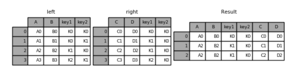
左连接:
result = pd.merge(left, right, how='left', on=['key1', 'key2'])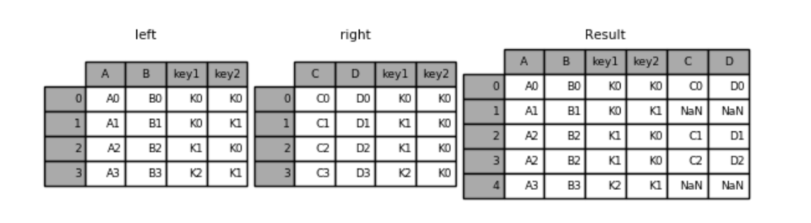
右连接:
result = pd.merge(left, right, how='right', on=['key1', 'key2'])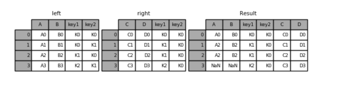
外连接:
result = pd.merge(left, right, how='outer', on=['key1', 'key2'])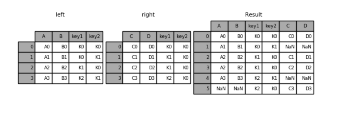
pd.join(df1, df2, how="inner"): 横向拼接,how 默认为 inner,可以指定 left,right,outer。
Pandas 数据分组与聚合
df.groupby(by): 按什么列分组,如果有多个列,需要传列表。
import pandas as pd

df = pd.DataFrame({
    "name": ["Alice", "Bob", "Charlie", "David", "Eve", "Frank"],
    "sex": ["F", "M", "F", "M", "F", "M"],
    "city": ["New York", "New York", "New York", "Chicago", "Chicago", "Chicago"],
    "score": [25, 30, 35, 40, 45, 50]
})

sex_group = df.groupby('sex')
city_group = df.groupby('city')

print(f"sex_group: \n{sex_group.head()}\n")
print(f"city_group: \n{city_group.head()}\n")

print(f"sex_group的类型: {type(sex_group)}")
print(f"sex_group中name列的类型: {type(sex_group['name'])}")
print(f"sex_group中F组的类型: {type(sex_group.get_group('F'))}\n")

sex_city_group = df.groupby(['sex', 'city'])
print(f"sex_city_group: \n{sex_city_group.head()}")
sex_group:
name sex city score
0 Alice F New York 25
1 Bob M New York 30
2 Charlie F New York 35
3 David M Chicago 40
4 Eve F Chicago 45
5 Frank M Chicago 50
city_group:
name sex city score
0 Alice F New York 25
1 Bob M New York 30
2 Charlie F New York 35
3 David M Chicago 40
4 Eve F Chicago 45
5 Frank M Chicago 50
sex_group的类型: <class 'pandas.api.typing.DataFrameGroupBy'>
sex_group中name列的类型: <class 'pandas.api.typing.SeriesGroupBy'>
sex_group中F组的类型: <class 'pandas.DataFrame'>
sex_city_group:
name sex city score
0 Alice F New York 25
1 Bob M New York 30
2 Charlie F New York 35
3 David M Chicago 40
4 Eve F Chicago 45
5 Frank M Chicago 50group() 的示例操作:
import pandas as pd

df = pd.DataFrame({
    "name": ["Alice", "Bob", "Charlie", "David", "Eve", "Frank", "Grace", "Heidi"],
    "sex": ["F", "M", "F", "M", "F", "M", "F", "M"],
    "city": ["New York", "New York", "New York", "Chicago", "Chicago", "Chicago", "Chicago", "Chicago"],
    "score": [25, 30, 35, 40, 45, 50, 55, 60],
    "grade": [1, 2, 1, 2, 3, 1, 3, 2]
})

print(f"按性别分组,计算男女生最高分: \n{df.groupby('sex').score.max()}\n")
# 还可以使用 df.groupby('sex').score.agg('max') 和 df.groupby('sex').agg({'score': 'max'})
print(f"按性别城市分组,计算每个城市的最高分: \n{df.groupby(['sex', 'city']).score.max()}\n")
# 还可以使用 df.groupby(['sex', 'city']).score.agg('max') 和 df.groupby(['sex', 'city']).agg({'score': 'max'})
print(f"按性别和城市分组,计算每个城市的最高年级和最高分: \n{df.groupby(['sex', 'city']).agg({'grade': 'max', 'score': 'max'})}\n")
按性别分组,计算男女生最高分:
sex
F 55
M 60
Name: score, dtype: int64
按性别城市分组,计算每个城市的最高分:
sex city
F Chicago 55
New York 35
M Chicago 60
New York 30
Name: score, dtype: int64
按性别和城市分组,计算每个城市的最高年级和最高分:
grade score
sex city
F Chicago 3 55
New York 1 35
M Chicago 2 60
New York 2 30使用透视表:
import pandas as pd

df = pd.DataFrame({
    "name": ["Alice", "Bob", "Charlie", "David", "Eve", "Frank", "Grace", "Heidi"],
    "sex": ["F", "M", "F", "M", "F", "M", "F", "M"],
    "city": ["New York", "New York", "New York", "Chicago", "Chicago", "Chicago", "Chicago", "Chicago"],
    "score": [25, 30, 35, 40, 45, 50, 55, 60],
    "grade": [1, 2, 1, 2, 3, 1, 3, 2]
})

print(f"按性别分组,计算男女生最高分: \n{df.pivot_table(index='sex', values='score', aggfunc='max')}\n")
print(f"按性别城市分组,计算每个城市的最高分: \n{df.pivot_table(index=['sex', 'city'], values='score', aggfunc='max')}\n")
print(f"按性别和城市分组,计算每个城市的最高年级和最高分: \n{df.pivot_table(index=['sex', 'city'], values=['grade', 'score'], aggfunc={'grade': 'max', 'score': 'max'})}\n")
按性别分组,计算男女生最高分:
score
sex
F 55
M 60
按性别城市分组,计算每个城市的最高分:
score
sex city
F Chicago 55
New York 35
M Chicago 60
New York 30
按性别和城市分组,计算每个城市的最高年级和最高分:
grade score
sex city
F Chicago 3 55
New York 1 35
M Chicago 2 60
New York 2 30df.filter(func): 过滤符合条件的数据。
# 需求: 按照城市分组, 查询每组销售金额平均值 大于 200的全部数据.
# filter(): 根据条件, 筛选出合法的数据.
# 换成SQL思路: select * from df where city in (select city from df group by city having avg(revenue) > 200);
df.groupby('city').filter(lambda s: s['revenue'].mean() > 200)
# df.groupby('city')['revenue'].filter(lambda s: s.mean() > 200)
Pandas 学习常见问题
Pandas 如何处理 None 和 NaN
- NaN (Not a Number) 来自 NumPy,是一个 浮点类型的特殊值。
- None 来自 Python,是一个 对象类型的空值。
在大多数 Pandas 场景中,None 会被自动识别为缺失,NaN 会被自动识别为缺失,isna/isnull 都能同时识别它们。
真正决定它们谁留下的是 dtype。
如果是数值列:
s = pd.Series([1, None, 3])
print(s.dtype) # float64
因为数值列 + None → Pandas 会把 None 自动转成 NaN,整列升级为 float64 (因为 NaN 只能存在于浮点里)。
s = pd.Series(["a", None, "b"]) # object如果是这样的,dtype 会被识别为 object,None 保持 None,不会强制变成 NaN,但仍然被 isna () 识别为缺失。
Pandas 的 axis = 0 什么时候是行,什么时候是列
DataFrame 像一个二维坐标系一样,axis 指的是计算/压缩/遍历发生的方向,而结果作用在剩下的那个维度上。
axis=0:跨行,对每一列做事。axis=1: 跨列,对每一行做事。
axis 从来不表示 "我要操作行还是列",它只表示 "我沿着哪条轴把数据压扁"。
举个例子:
import pandas as pd

df = pd.DataFrame({
    "A": [1, 2, 3],
    "B": [4, 5, 6]
})
表结构:
   A  B
0  1  4
1  2  5
2  3  6
如果我们用 df.sum(axis=0) 求和,结果是:
A    6
B   15
这是因为 axis=0 表示 "按列求和",所以 A 和 B 两列被求和了。nih1
你好如果我们用 df.sum(axis=1) 求和,结果是:
0     5
1     7
2     9
如果我们用 df.drop("A", axis=1), axis = 1 的真实含义是: "按列删除",所以删除的是列,而不是 axis = 1 就是列,而是因为 你在 columns 这条轴上做结构变化。
Matplotlib
Matplotlib 可以把它看成 Python 世界里的“老牌绘图引擎”。如果数据需要变成图,它通常是第一批被请上场的工具之一。设计目标很直接:把数据变成可视化结果,而且尽量接近 MATLAB 的使用体验,所以名字里就有个 “mat”。
它的核心能力是二维绘图:折线图、散点图、柱状图、直方图、饼图、热力图这些基础图形都能稳定产出。底层是面向对象的绘图系统,上层又提供了一个接近“命令式脚本风格”的接口(pyplot)。多数人先用 pyplot,因为写起来像这样一路画下去,心智负担小;等需要精细控制时,再切换到面向对象接口去精调坐标轴、子图、刻度、样式。
典型工作流程很朴素:准备数据 → 创建图和坐标轴 → 调用绘图函数 → 调整样式 → 显示或保存。它和 NumPy、Pandas 贴合度很高,数组或 Series 往里一塞就能画。很多高级可视化库(比如 seaborn)本质上也是在 Matplotlib 上包了一层“更省心的语法糖”。
Matplotlib 绘图示例
绘制一个图,需要导入 matplotlib.pyplot 模块,然后设置中文字体,准备数据,
import matplotlib.pyplot as plt

plt.rcParams["font.family"] = ["Times New Roman", "SimSun"]  # 英文字体为新罗马,中文字体为宋体
plt.rcParams["font.serif"] = ["Times New Roman", "SimSun"]  # 衬线字体
plt.rcParams["font.sans-serif"] = ["Times New Roman", "SimSun", "Arial", "SimHei"]  # 无衬线字体,与Latex相关
plt.rcParams["mathtext.fontset"] = "custom"  # 设置LaTeX字体为用户自定义,这里演示,就不用computer modern了
plt.rcParams["axes.unicode_minus"] = False

plt.figure(figsize=(10, 5), dpi=200)  # 创建画布

x = [i for i in range(1, 25)]  # X轴信息
y = [-8, -8, -8, -7, -7, -7, -6, -6, -7, -5, -4, -1, 1, 1, 2, 1, -1, -4, -4, -5, -5, -6, -7, -7]

x_labels = [f"{i:2d}:00" for i in x[::2]]
y_labels = [f"{i}℃" for i in y]

plt.plot(x, y, linewidth=1)
plt.xticks(x[::2], x_labels)
plt.yticks(y, y_labels)
plt.title("沈阳24小时气温变化", pad=10)
plt.xlabel("时间", labelpad=10)
plt.ylabel("气温", labelpad=10)
plt.grid(True, linestyle="--", linewidth=0.5)

plt.show()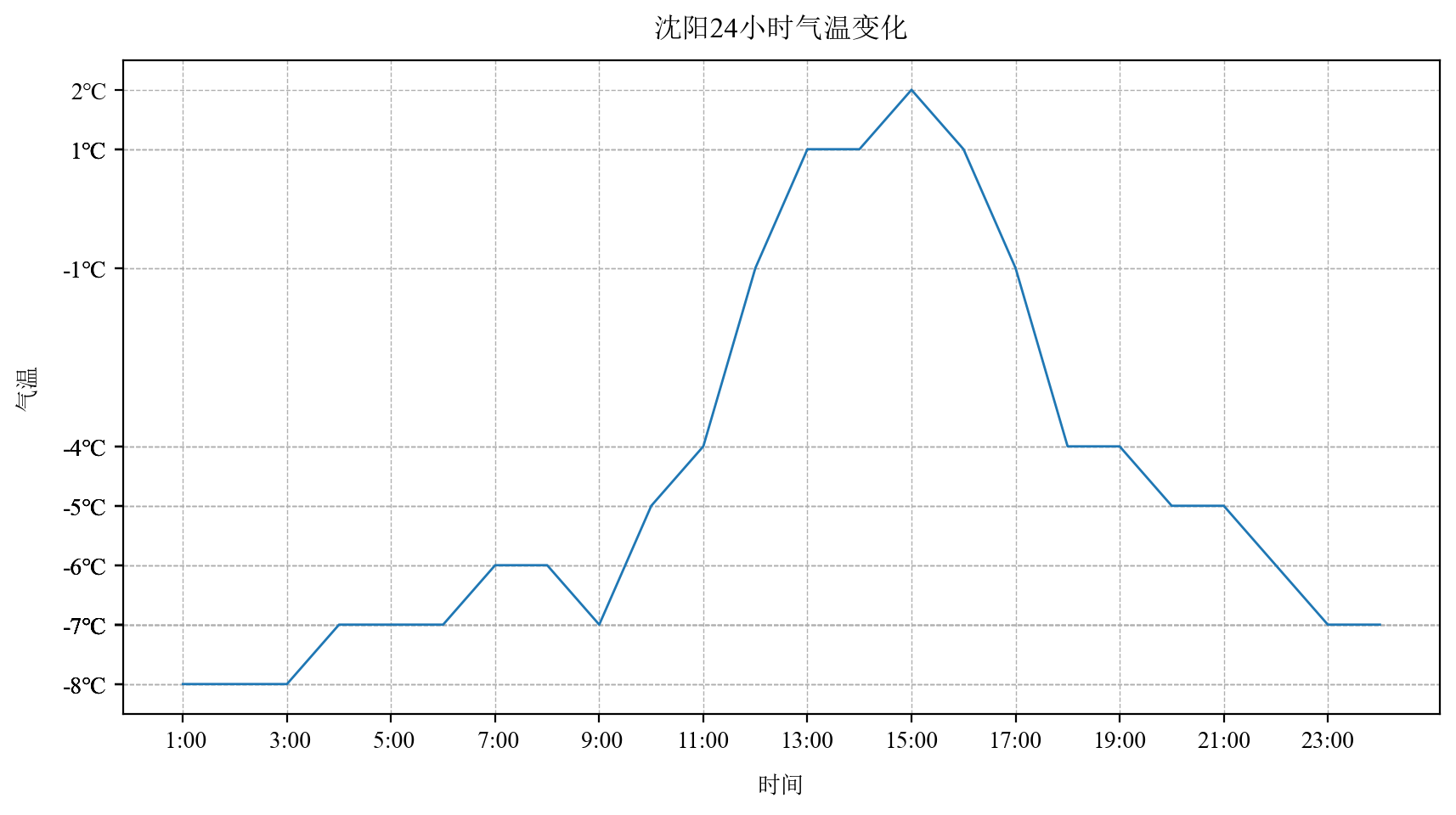
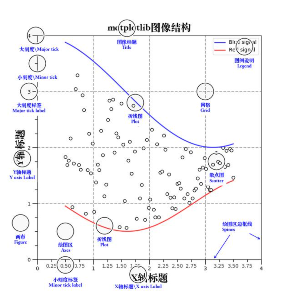
Matplotlib 图形结构
可结合上一个图形对比查看。
Matplotlib 图形种类
折线图
matplotlib.pyplot.plot(x, y, ...): 绘制折线图,用于展示数据随时间或类别的变化趋势。
常用参数:
x, y: x 轴和 y 轴的数据序列color/c: 线条颜色,支持颜色名称('r' 红色、'b' 蓝色)或十六进制('#FF5733')linestyle/ls: 线条样式,'-' 实线、'--' 虚线、':' 点线、'-.' 点划线linewidth/lw: 线条宽度,默认 1.0marker: 标记点样式,'o' 圆点、's' 方块、'^' 上三角、'd' 菱形、'x' 叉号markersize/ms: 标记点大小markerfacecolor/mfc: 标记点填充颜色markeredgecolor/mec: 标记点边缘颜色alpha: 透明度,0-1 之间的值label: 图例标签,配合plt.legend()使用
import random
import matplotlib.pyplot as plt

plt.figure(figsize=(10, 5), dpi=100)

x = [i for i in range(1, 11)]
y1 = [random.uniform(3, 5) for i in range(10)]
y2 = [random.uniform(4, 6) for i in range(10)]

plt.plot(x, y1, color='steelblue', linestyle='--', linewidth=2,
         marker='o', markersize=6, label='Series A')
plt.plot(x, y2, color='#FF6B6B', linestyle='-', linewidth=2,
         marker='s', markersize=6, label='Series B')
plt.ylim(2, 8)
plt.legend()

plt.show()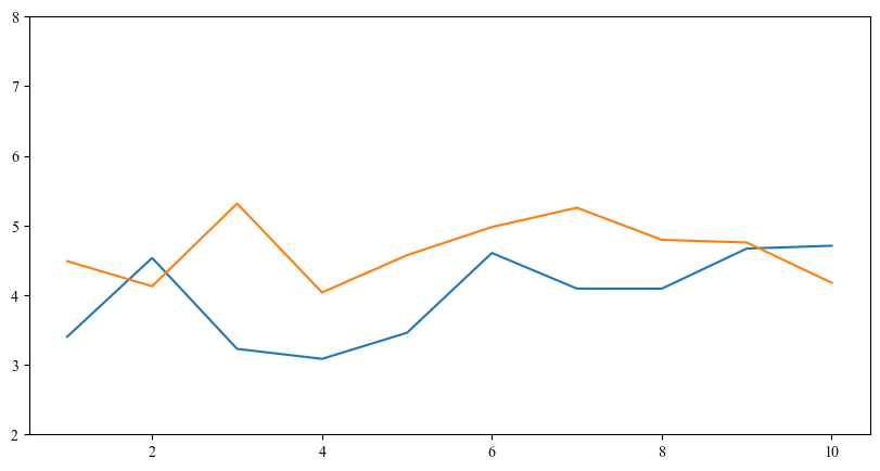
柱状图
matplotlib.pyplot.bar(x, height, ...): 绘制柱状图,用于比较不同类别的数值大小。
常用参数:
x: 柱子的 x 轴位置height: 柱子的高度width: 柱子宽度,默认 0.8bottom: 柱子底部的 y 坐标,用于堆叠柱状图color/c: 柱子颜色edgecolor/ec: 柱子边缘颜色linewidth/lw: 边缘线宽alpha: 透明度align: 柱子对齐方式,'center'(默认)或 'edge'label: 图例标签hatch: 填充纹理,'/' 斜线、'\' 反斜线、'x' 交叉线、'.' 点状
import random
import matplotlib.pyplot as plt

plt.figure(figsize=(10, 5), dpi=100)

x = [i for i in range(1, 11)]
y1 = [random.randint(1, 101) for i in range(10)]

plt.bar(x, y1, width=0.6, color='skyblue', edgecolor='navy',
        linewidth=1.2, alpha=0.8, label='Value')
plt.ylim(0, 100)
plt.legend()

plt.show()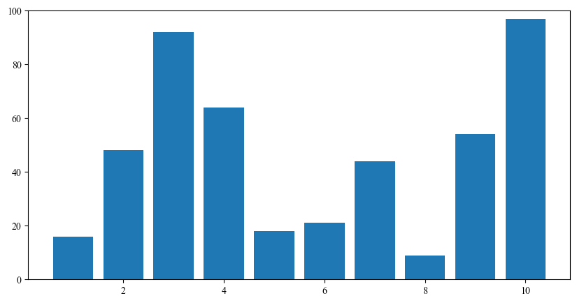
直方图
matplotlib.pyplot.hist(x, ...): 绘制直方图,用于展示数据的分布情况。
常用参数:
x: 输入数据序列bins: 柱子数量或边界,可以是整数、序列或字符串('auto'、'fd'、'doane'、'scott'、'stone'、'rice'、'sturges'、'sqrt')range: 数据范围,元组 (min, max)density: 是否归一化为概率密度,默认 Falseweights: 每个数据点的权重cumulative: 是否绘制累积分布,默认 Falsebottom: 柱子底部的 y 坐标histtype: 直方图类型,'bar'(默认并列)、'barstacked'(堆叠)、'step'(阶梯)、'stepfilled'align: 柱子对齐,'left'、'mid'(默认)、'right'orientation: 方向,'vertical'(默认)或 'horizontal'color/c: 柱子颜色edgecolor/ec: 边缘颜色linewidth/lw: 边缘线宽alpha: 透明度
import numpy as np
import matplotlib.pyplot as plt

# 生成随机数据(正态分布)
data = np.random.randn(1000)

plt.figure(figsize=(10, 5), dpi=100)

plt.hist(data, bins=30, color='steelblue', edgecolor='black',
         linewidth=0.8, alpha=0.7, density=True)

plt.show()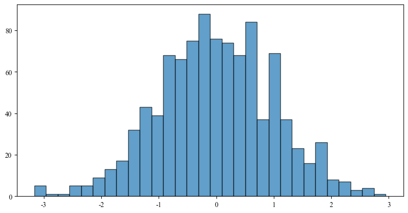
饼图
matplotlib.pyplot.pie(x, ...): 绘制饼图,用于展示各部分占整体的比例。
常用参数:
x: 各扇形的数值(自动计算比例)explode: 扇形偏离圆心的距离数组,用于突出显示某块labels: 各扇形的标签colors: 扇形颜色列表autopct: 百分比显示格式,如 '%1.1f%%' 显示一位小数pctdistance: 百分比文本距圆心的距离,默认 0.6shadow: 是否添加阴影,默认 Falselabeldistance: 标签距圆心的距离,默认 1.1startangle: 起始角度,默认从 x 轴正方向逆时针radius: 饼图半径,默认 1counterclock: 是否逆时针绘制,默认 Truewedgeprops: 扇形属性字典,如textprops: 文本属性字典center: 饼图中心位置,默认 (0, 0)frame: 是否绘制坐标轴框架,默认 False
import matplotlib.pyplot as plt

# 饼图数据
labels = ['Apple', 'Banana', 'Orange', 'Grape', 'Mango']
sizes = [30, 20, 15, 25, 10]
colors = ['#ff9999', '#66b3ff', '#99ff99', '#ffcc99', '#ff99cc']
explode = [0, 0, 0, 0.1, 0]  # 突出显示 Grape

plt.figure(figsize=(8, 8), dpi=100)

plt.pie(sizes, explode=explode, labels=labels, colors=colors,
        autopct='%1.1f%%', startangle=90,
        wedgeprops={'linewidth': 1, 'edgecolor': 'white'},
        textprops={'fontsize': 12})

plt.title('Pie Chart Example')

plt.show()
散点图
matplotlib.pyplot.scatter(x, y, ...): 绘制散点图,用于展示两个变量之间的关系。
常用参数:
x, y: 点的 x 和 y 坐标s: 点的大小,可以是标量或与数据等长的数组c/color: 点的颜色,可以是颜色、颜色列表或与数据等长的数组(配合 cmap 使用)marker: 标记样式,'o' 圆点、's' 方块、'^' 三角、'd' 菱形、'p' 五边形、'*' 星形cmap: 颜色映射,当 c 为数组时使用,如 'viridis'、'plasma'、'coolwarm'、'jet'alpha: 透明度,0-1 之间的值linewidths/lw: 标记边缘线宽edgecolors/ec: 标记边缘颜色label: 图例标签vmin, vmax: 颜色映射的范围norm: 颜色归一化对象
import numpy as np
import matplotlib.pyplot as plt

# 生成随机数据
np.random.seed(42)
x = np.random.randn(100)
y = np.random.randn(100)
colors = np.random.rand(100)
sizes = np.random.rand(100) * 300

plt.figure(figsize=(10, 6), dpi=100)

plt.scatter(x, y, c=colors, s=sizes, alpha=0.6, cmap='viridis',
           edgecolors='black', linewidths=0.5)

plt.xlabel('X Axis')
plt.ylabel('Y Axis')
plt.title('Scatter Plot Example')
plt.colorbar(label='Color Value')

plt.show()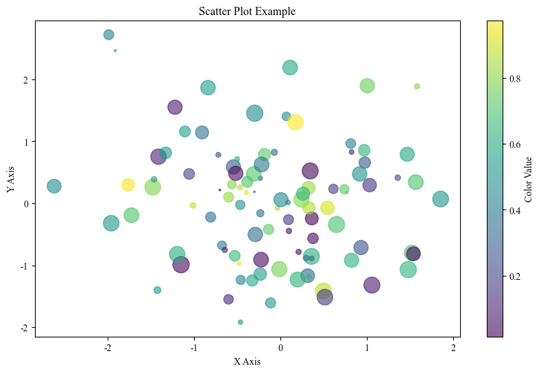
Matplotlib 辅助绘图
plt.xticks(ticks=None, labels=None, **kwargs):设置或获取横轴刻度,作用是控制 x 轴“刻度位置”和“刻度显示文字”。
常见用法有三种层级:
1)只设置刻度位置
plt.xticks([0, 1, 2, 3, 4])2)同时设置位置 + 显示标签
plt.xticks(
    [0, 1, 2, 3],
    ["10:00", "10:30", "11:00", "11:30"]
)
3)控制刻度样式(通过 kwargs)
plt.xticks(
    [0, 1, 2, 3],
    fontsize=12,
    rotation=45   # 旋转角度,时间标签常用
)
常用参数说明:
- ticks:刻度位置列表
- labels:刻度文字列表(长度必须和 ticks 一致)
- rotation:旋转角度
- fontsize:字体大小
- color:刻度文字颜色
同理:
plt.yticks(...):设置或获取纵轴刻度。 参数和 xticks 完全同构,行为一致,只是作用在 y 轴。
plt.grid(True, linestyle='--', alpha=0.5):显示网格线
作用是提高读图精度,让视觉系统更容易估计数值位置。
常见参数:
plt.grid(
    True,              # 是否显示
    linestyle='--',    # 线型:'-' '--' '-.' ':'
    linewidth=1,       # 线宽
    color='gray',      # 颜色
    alpha=0.5          # 透明度
)
进阶用法:只开某个方向的网格
plt.grid(axis='x')   # 只显示竖向网格
plt.grid(axis='y')   # 只显示横向网格
plt.xlabel() / plt.ylabel():设置坐标轴名称
plt.xlabel("时间", fontsize=14)
plt.ylabel("温度(℃)", fontsize=14)
常见参数:
- fontsize:字号
- labelpad:与轴的间距
- loc:位置(left / right / center,较新版本支持)
plt.title():设置图标题
plt.title(
    "中午11点到12点温度变化",
    fontsize=20,
    loc='center'
)
可用参数:
- fontsize:字号
- loc:位置(left / center / right)
- pad:和图像的间距
多语言环境经常遇到一个现实问题:中文可能乱码。那是字体问题,需要先设置中文字体,否则 matplotlib 默认字体库不含中文字符。
plt.savefig("test.png"):保存图片到文件。
这是绘图流程里的“落盘指令”,不调用就只会显示,不会保存。
常用增强参数:
plt.savefig(
    "test.png",
    dpi=300,              # 分辨率(打印/论文必调)
    bbox_inches="tight",  # 去掉多余白边
    transparent=False     # 是否透明背景
)
关键细节顺序规则:
先 savefig,再 show。
plt.savefig("test.png")
plt.show()
因为在某些后端环境里,show() 会清空当前图像缓冲区,导致保存到空图。
Matplotlib 常见问题
中文显示方块
这是 Matplotlib 没有正确加载字体导致的,在导入 Matplotlib 后添加如下代码即可。
plt.rcParams["font.family"] = ["Times New Roman", "SimSun"]  # 英文字体为新罗马,中文字体为宋体
plt.rcParams["font.serif"] = ["Times New Roman", "SimSun"]  # 衬线字体
plt.rcParams["font.sans-serif"] = ["Times New Roman", "SimSun", "Arial", "SimHei"]  # 无衬线字体,与Latex相关
plt.rcParams["mathtext.fontset"] = "custom"  # 设置LaTeX字体为用户自定义,这里演示,就不用computer modern了
plt.rcParams["axes.unicode_minus"] = False
版权所有
版权归属: